|
 |
|
This tutorial demonstrates how to collect, filter and plot tweets using the R rtweet package.
The rtweet package has been designed by Michael W. Kearney to collect and organise Twitter data using Twitter’s Application Program Interfaces (API). Further details about the package can be found at:
# install.packages("pacman")
pacman::p_load(tidyverse, tidytext, rtweet)

library(tidyverse)
library(ggplot2)
library(tidytext)
library(rtweet)
library(knitr)
Let’s search for tweets with the hash-tag #StarWars. In this query (q) we are searching with the hash tag #StarWars, we will take a total(n) of up to 1800 tweets, we are not interested in retweets or replies to tweets, and we are looking for tweets in English (lang).
tweets <- search_tweets(q = "#StarWars",
                       n = 18000,
                       include_rts = FALSE,
                       `-filter` = "replies",
lang = "en")Check the first 10 tweets and then export them all as a CSV file.
tweets %>%
  head(10) %>%
  select(created_at, screen_name, text, favorite_count, retweet_count)
## # A tibble: 10 x 5
## created_at screen_name text favorite_count retweet_count
## <dttm> <chr> <chr> <dbl> <dbl>
## 1 2020-06-25 20:39:49 DanTheGreat… "When you come… 0 1
## 2 2020-06-25 20:39:10 jaychocnh "We ready now … 0 0
## 3 2020-06-25 20:39:10 jaychocnh "Mark 1 month … 0 0
## 4 2020-06-24 23:00:46 jaychocnh "My Charizard … 0 0
## 5 2020-06-24 22:51:07 jaychocnh "Somebody from… 0 0
## 6 2020-06-25 20:38:23 swcutscenes "Watch #StarWa… 0 0
## 7 2020-06-25 20:38:23 swcutscenes "Here is #cine… 0 0
## 8 2020-06-25 13:47:07 swcutscenes "Like our Face… 0 0
## 9 2020-06-25 03:42:39 swcutscenes "Only on https… 0 0
## 10 2020-06-24 17:33:10 swcutscenes "Exclusive #St… 0 0Why don’t we save all these tweets as a CSV file
write_as_csv(tweets, "StarWars-tweets.csv")Let’s look at the timeline of our tweets
ts_plot(tweets, "hours") +
  labs(x = NULL, y = NULL,
       title = "Frequency of tweets with a #StarWars hashtag",
       subtitle = paste0(format(min(tweets$created_at), "%d %B %Y"), " to ", format(max(tweets$created_at),"%d %B %Y")),
       caption = "Data collected from Twitter's REST API via rtweet") +
  ggplot2::theme_classic()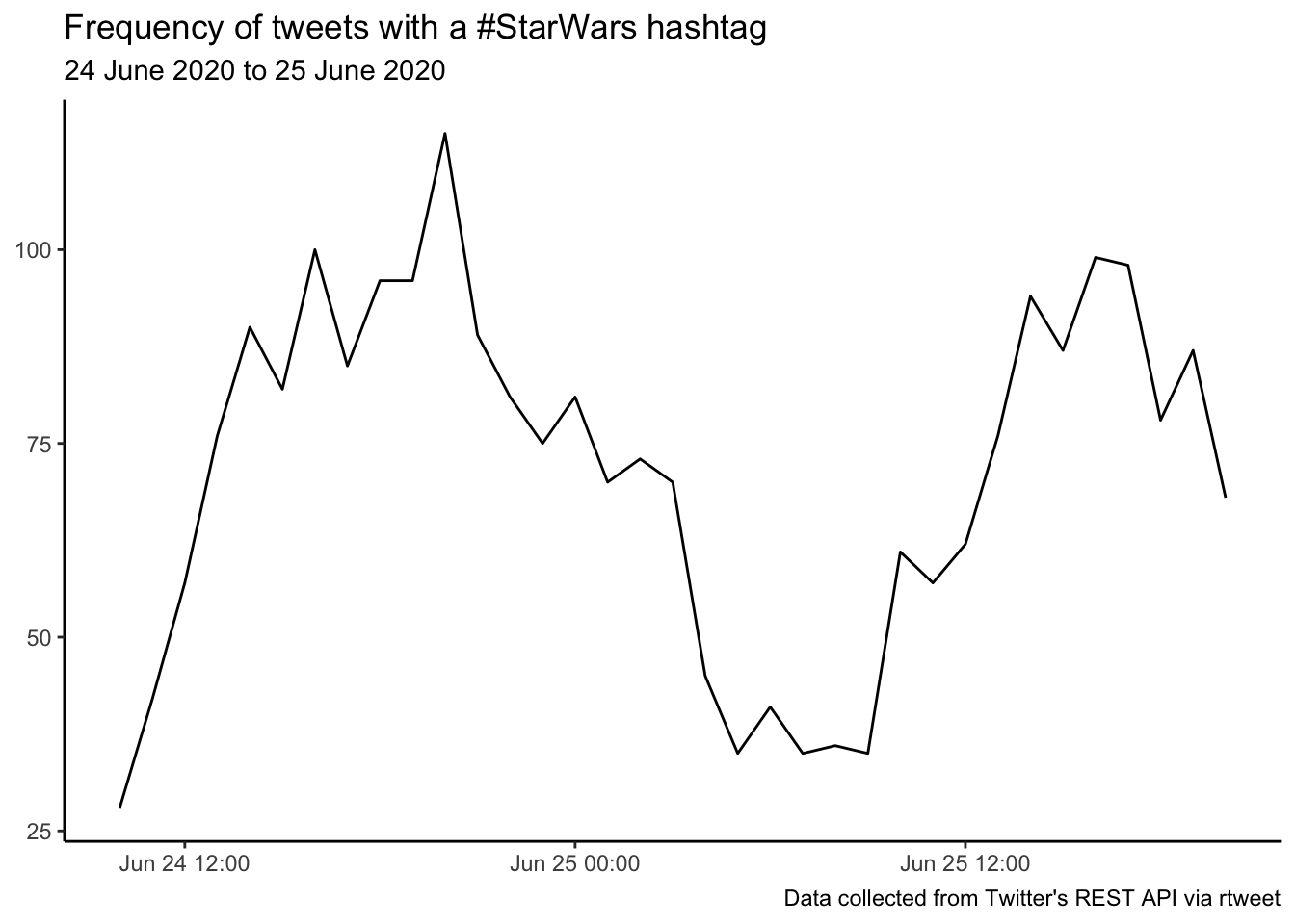
What was the top tweeting location
tweets %>%
  filter(!is.na(place_full_name)) %>%
  count(place_full_name, sort = TRUE) %>%
  top_n(5)
## # A tibble: 5 x 2
## place_full_name n
## <chr> <int>
## 1 Maryland, USA 6
## 2 San Francisco, CA 5
## 3 Salford, England 4
## 4 Louisville, KY 3
## 5 Zutphen, Nederland 3The most retweeted tweet
tweets %>%
  arrange(-retweet_count) %>%
  slice(1) %>%
  select(created_at, screen_name, text, retweet_count)
## # A tibble: 1 x 4
## created_at screen_name text retweet_count
## <dttm> <chr> <chr> <dbl>
## 1 2020-06-24 16:09:54 RamenDoodles… *Aggressive cuddling*! Saw tw… 1098The most liked tweet
tweets %>%
  arrange(-favorite_count) %>%
  top_n(5, favorite_count) %>%
  select(created_at, screen_name, text, favorite_count)
## # A tibble: 5 x 4
## created_at screen_name text favorite_count
## <dttm> <chr> <chr> <dbl>
## 1 2020-06-24 15:56:31 thisuserisan… "Gender swap AU (just obi-wa… 6753
## 2 2020-06-24 16:09:54 RamenDoodles… "*Aggressive cuddling*! Saw … 3944
## 3 2020-06-24 19:22:41 starwars "It’s The #StarWarsShow! Thi… 1623
## 4 2020-06-24 21:10:21 TheSWU "‘The Rise Of Skywalker’ art… 1170
## 5 2020-06-25 13:22:43 PhilSzostak "“A little after hours proje… 983Who were the top tweeters
tweets %>%
  count(screen_name, sort = TRUE) %>%
  top_n(10) %>%
  mutate(screen_name = paste0("@", screen_name))
## # A tibble: 10 x 2
## screen_name n
## <chr> <int>
## 1 @bpdstarwars 124
## 2 @FanthaTracks 30
## 3 @StarWarsRP 27
## 4 @tpnalliance 27
## 5 @rcmadiax 24
## 6 @ST4RW4RS 22
## 7 @JediNewsNetwork 21
## 8 @AnakinS03737461 17
## 9 @VintageStarWars 16
## 10 @ClassicStarWars 10What was the most used emoji
# install.packages("devtools")
devtools::install_github("hadley/emo")

library(emo)
tweets %>%
  mutate(emoji = ji_extract_all(text)) %>%
  unnest(cols = c(emoji)) %>%
  count(emoji, sort = TRUE) %>%
  top_n(10)
## # A tibble: 10 x 2
## emoji n
## <chr> <int>
## 1 🔗 128
## 2 😍 35
## 3 😂 30
## 4 🤣 29
## 5 👉 28
## 6 ❤️ 20
## 7 🚨 16
## 8 😎 15
## 9 👍 14
## 10 😁 14What were the top 10 hashtags
tweets %>%
  unnest_tokens(hashtag, text, "tweets", to_lower = FALSE) %>%
  filter(str_detect(hashtag, "^#"),
         hashtag != "#StarWars") %>%
  count(hashtag, sort = TRUE) %>%
  top_n(10)
## # A tibble: 12 x 2
## hashtag n
## <chr> <int>
## 1 #starwars 809
## 2 #eBay 135
## 3 #TheMandalorian 86
## 4 #Disney 47
## 5 #marvel 45
## 6 #STARWARS 45
## 7 #Starwars 43
## 8 #topps 41
## 9 #babyyoda 40
## 10 #darthvader 39
## 11 #disney 39
## 12 #LEGO 39Top mentions
tweets %>%
  unnest_tokens(mentions, text, "tweets", to_lower = FALSE) %>%
  filter(str_detect(mentions, "^@")) %>%
  count(mentions, sort = TRUE) %>%
  top_n(10)
## # A tibble: 11 x 2
## mentions n
## <chr> <int>
## 1 @starwars 51
## 2 @YouTube 26
## 3 @HamillHimself 23
## 4 @Disney 20
## 5 @Poshmarkapp 14
## 6 @EAStarWars 11
## 7 @StarWars 11
## 8 @eBay 10
## 9 @Hasbro 9
## 10 @LEGOGroup 9
## 11 @themandalorian 9Let’s examine the most frequently used words in these tweets
words <- tweets %>%
mutate(text = str_remove_all(text, "&|<|>"),
text = str_remove_all(text, "\\s?(f|ht)(tp)(s?)(://)([^\\.]*)[\\.|/](\\S*)"),
text = str_remove_all(text, "[^\x01-\x7F]")) %>%
unnest_tokens(word, text, token = "tweets") %>%
filter(!word %in% stop_words$word,
!word %in% str_remove_all(stop_words$word, "'"),
str_detect(word, "[a-z]"),
!str_detect(word, "^#"),
!str_detect(word, "@\\S+")) %>%
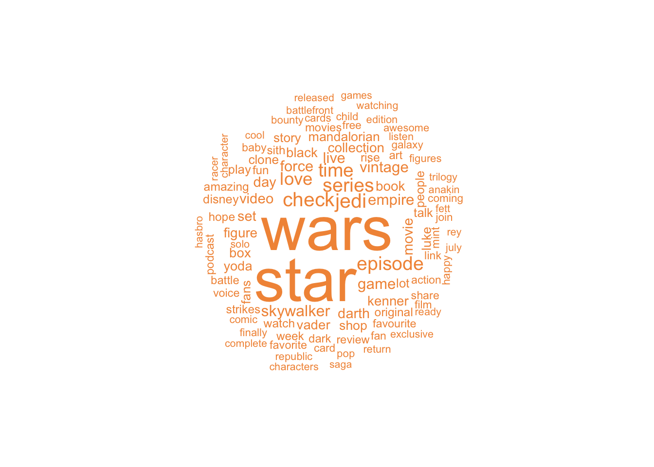
count(word, sort = TRUE)Finally - let’s use the wordcloud package to create a visualisation of the word frequencies.
library(wordcloud)
words %>%
  with(wordcloud(word, n, random.order = FALSE, max.words = 100, colors = "#F29545"))